Google 20 for 1 stock split

Google announced Tuesday its results for Q4 2021 and that they plan to split shares at 20 for 1 this Tuesday. Basically, if you are a shareholder, for each 1 share of Google at (about) 3000$ dollars you will have (at the ex-date) 20 shares at 150$.

Nothing should really change, but there might be some financial effects, for instance, due to the inclusion of the stock in new indices or increased market liquidity.

It’s a good story in the end: more small investors can now afford to get a share of Google, so the stock is more valuable.

Is there any impact on the stock price¹ and can it be measured in this specific case?

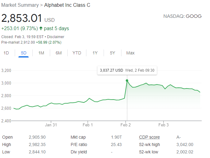
The question was inspired by a few headlines juxtaposing the stock split itself with the very good performance that the stock achieved² in the same day, which increased by about 7%.

So was the 7% daily return due to the split announcement? This is the question we’ll try to investigate here by building a naive counterfactual.

The idea of constructing a counterfactual, i.e. this way of thinking, came originally by reading the book “the causal mixtape” (J. Cunningham) and is being put into practice just for fun. If you want to take a single takeaway from this post, here it is: get a copy of the book =).

A naive counterfactual model

A counterfactual model will help us in reframing the question in the following terms: what would have happened if Google did not release this announcement? I am taking here the announcement as a whole, this is important and we’ll soon go back to this: the idea is to get a sense of how “special” has last Tuesday been when compared to what happens “normally”.

It is assumed that the return of the google stock at any given (end-of) day is determined by the return of other - similar - stocks plus some factors that are idiosyncratic to Google, those factors making the company unique. Let us try to build a model that quantifies the return of GOOG as a function of other ones, assuming that the errors of this model are due to the idiosyncrasies of the Google stock.

So we are assuming a priori that Google returns can be explained by the returns of other selected tech companies, namely: Microsoft, Facebook, Amazon, Apple are clear candidates, but I’ll add also Nvidia, Twitter, Tesla, Adobe, Etsy, Garmin and Oracle. None of these companies is exactly like Google with its unique mix of revenue sources (search) and experiments (minor exposure to cloud, hardware, autonomous car, robots).

However, at the end of the day, we are just interested in determining how much do the returns of these companies tell about Google’s return. If we are able to explain Google returns in this fashion, we can then compare the hypothetical “no announcement” estimated return to the actual one that the stock achieved on Tuesday.

Data sourcing

skip over this section if you’re not interested in replicating the analysis.

This is the easy part: daily stock data can be obtained from several sources. I choose alphavantage, getting a free key. If you want to replicate the experiment, I suggest using the python library alpha_vantage with pandas: pip install alpha_vantage pandas.

Notice that the free version gives you a limited amount of requests, so we must wait a little time between requests:

# Set ALPHAVANTAGE_TOKEN, install requirements
from alpha_vantage.timeseries import TimeSeries
import pandas as pd
import time
ts = TimeSeries(key=ALPHAVANTAGE_TOKEN,output_format='pandas', indexing_type='date')
def get_pd_data(tickers=["GOOGL"], outputsize="compact"):
  dfs = []
  for i,t in enumerate(tickers):
    if (i%4)==0 and i>0:
      print(f"{i} Pausing for 65 s")
      time.sleep(65)
      
    data, meta_data = ts.get_daily(t, outputsize=outputsize)
    data["price"] = data['4. close']
    data["ticker"] = t
    dfs.append(data.reset_index().set_index(["ticker","date"]))
  
  print("Done")
  return pd.concat(dfs, axis=0)

# GOOG are C shares, while GOOGL are A shares (w voting rights)
tickers = ["GOOG","MSFT","FB","AMZN","ETSY","GRMN","ADBE","AAPL","NVDA","TWTR","TSLA","ORCL"]
data = get_pd_data(tickers=tickers, outputsize="full")
d = data.reset_index().query("date>'2016-01-01'")[["ticker","date","price"]]

We are basically taking the data for all the mentioned stocks from 2016 onward. How does this look?

Looking at the plot, you may notice that Google is not the only company that has been recently interested by stock splits: so did NVDA, AAPL, TSLA.

For this reason, we’ll remove from the dataset those days where computing returns from the face value would be wrong³: 2021-07-20 (because of NVDA), 2020-08-31 (TSLA and AAPL).

So, how do return from other companies explain GOOG returns?

Let’s run a simple linear regression on data from Jan 1st, 2016 to December 31, 2021. The following weights are obtained, linking google returns to the returns of other stocks:

R^2: 0.677. Fitted with data till 2021-12-31. Weights:
MSFT->  0.375
FB  ->  0.195
AMZN->  0.121
GRMN->  0.056
AAPL->  0.054
ADBE->  0.042
TWTR->  0.020
NVDA->  0.016
ORCL->  0.014
TSLA-> -0.005
ETSY-> -0.010

The results are pretty interesting: in the considered time frame MSFT,FB and AMZN get the most of the weight. Comparing the goodness-of-fit of a model on data it’s been trained on is questionable. Data in 2022 has not been used yet: let’s plot the predictions of our model (y-axis) vs the actual GOOG returns (y-axis).

Notice that the colors are used to discriminate whether the given datapoint has been used for calibrating the model parameters (blue) or not (red), while the different marker highlights last Tuesday.

The size of the point is the model error: hover to see the date when a given return was achieved. The overall R squared for the red points is 0.486. Points on the right-hand side of the xy bisector indicate a positive excess return for GOOG, when compared to the estimated one.

Considerations

A very simple model was built to assess if after the last Tuesday announcement an unusual amount of GOOG returns were unexplainable.

It can be seen from the plot that there indeed is about 6% of unexplained or “excess” return from last Tuesday with respect to other companies, but we are still left with the original question: is it due to the earnings or is there another effect?

Fact is: the announcement released on Tuesday did not carry only the stock split, but also the earnings report. Is this excess return due to the earnings or to the stock split and in which proportion?

Properly disentangling the two components requires a more sophisticated analysis, but even after this naive modelling, we can observe the suggestive similarity between this year (big red datapoint) and past year Google’s Q4 announcements in the same period (the big blue one), both having about 6% error with respect to the model.

If I had to bet, I’d bet against such an effect, especially for highly liquid stocks and capitalized companies like Google is, but that’s just an opinion.

One week later: update on Data distribution shift

So, this week I have added to my read list Chip’s Huyen post “Data Distribution Shifts and Monitoring”.

At first, I did not think of running any cross validation on this experiment for two reasons. Such a simple model is expected to capture basic relationships that are supposed to be stable in time.

Is this true tough? I started asking if I would have drawn the same conclusions if the model was built 6 months in advance, i.e. when trained till June, 2021. Since we have a very simple linear model let’s compare the model coefficient first. You know, one of the benefits of using simple linear models.

R^2: 0.681. Fitted with data to **2021-06-30**. Weights:

MSFT-> 0.343 (0.375, when fitting till 2021-12-31)
FB  ->  0.203 (0.195)
AMZN->  0.114 (0.121)
GRMN-> 0.066 (0.056)
AAPL-> 0.053 (0.054)
ADBE-> 0.058 (0.042)
TWTR-> 0.023 (0.020)
NVDA-> 0.014 (0.016)
ORCL-> 0.021 (0.014)
TSLA-> -0.004 (-0.005)
ETSY-> -0.009 (-0.010)

Good! Also changing the training period, we preseved the relationships! Let’s walk forward with this second model and see the test R^2 for each month (yellow), which turns to be comparable with the one we already got on the last month:  

Also the predictions look similar, as expected: